
Contents
- I. Detailed Explanation of Core Information of ulab
- 1.1 Positioning and Design Objectives of ulab
- 1.2 Firmware Customization (The Key to Reducing Size)
- 1.3 Compatibility with numpy
- 1.4 Version String Interpretation
- 1.5 Check Functions Supported by the Firmware
- II. Detailed Explanation of Core Knowledge Points of ndarray
- 2.1 Basic Features of ndarray
- 2.2 Array Initialization
- 2.3 Attributes and Methods of ndarray
- 2.4 Operator Usage Rules
- 2.5 Slicing and Indexing
- 3. Classification and Core Description of numpy Functions in ulab
- 3.1 Logical Judgment Category
- 3.2 Indexing and Sorting Category
- 3.3 Numerical Calculation Category
- 3.4 Array Operations
- 3.5 Bitwise Operations
- 3.6 Complex Number Related Classes
- 3.7 Matrix and Convolution Category
- 3.8 File IO Classes
- IV. ulab Library General Mathematical function
- 4.1 Common Rules for Basic General Functions
- 4.2 Exclusive Rules for Special General Functions
- 4.3 Custom function vectorization (np.vectorize)
- 4.4 Key Differences Between ulab Universal Functions and Standard NumPy
- 5. FFT/IFFT in ulab
- 5.1 Core Rules (Default Behavior When Plural Support Is Unavailable)
- 5.2 NumPy Compatibility Mode After Enabling Complex Number Support
- 5.3 Key Differences from Standard NumPy
- VI. The linalg Linear Algebra Module in ulab
- 6.1 Overview of function Features
- 6.2 In-depth Analysis of Key Functions
- 6.3 Core Differences Between ulab and numpy
- VII. Random Number Generation with ulab numpy.random
- 7.1 Basics: Generator Object
- 7.2 Three Major Random Number Methods: Comparison of Parameters and Functions
- 7.3 Key Usage Examples and Notes
- VIII. Integration with ulab scipy.integrate
- 8.1 Basic Module Configuration (Prerequisite: Must Be Met First)
- 8.2 Four Major Integral Functions: Comparison of Core Parameters and Characteristics
- 8.3 In-depth Analysis of Key Functions
- IX. Solving Linear Systems with ulab scipy.linalg
- 9.1 Core Comparison of Two Functions
- 9.2 In-depth Analysis of Key Functions
- X. Root Finding for Univariate Functions with ulab scipy.optimize
- 10.1 Core Comparison of the Three Major Functions
- 10.2 In-depth Analysis of Key Functions
- 10.3 Core Differences from CPython scipy
- 11. ulab scipy.signal.sosfilt Second-order IIR Filter
- 11.1 Brief Introduction
- 11.2 Core Differences from CPython scipy.signal.sosfilt
- 11.3 Application Example: Power Frequency Filtering
- 12. ulab scipy.special Special Mathematical Functions
- 13. ulab utils Module: Data Conversion and Spectrum Analysis
- 13.1 Module Enable Method (compile macro must be configured)
- 13.2 Core Functions
- 14. Core Optimization Techniques for ulab
- 14.1 Prefer using ndarray over native iterable objects
- 14.2 Choose a reasonable dtype (core to memory saving)
- 14.3 Optimize the Axis Order of Multidimensional Arrays (Place the Longest Axis at the End)
- 14.4 Reduce Intermediate Products (Avoid Memory Fragmentation)
- 14.5 Image/Array Scaling (Low-Resolution Sensor Adaptation)
- 15. A Brief Analysis of the Underlying Implementation and Extension of ulab
- Summary of links to relevant firmware, source code and documents
- Source Code
- ulab Firmware Download
- Document
- Version Record
I. Detailed Explanation of Core Information of ulab
1.1 Positioning and Design Objectives of ulab
ulab is a lightweight numpy/scipy subset built for MicroPython, optimized specifically for microcontroller use cases, with three core design objectives:
- Real-time performance: Microcontrollers need to process peripheral data in a timely manner (e. g., performing FFT on signals acquired by the ADC), and ulab is 30-50 times faster than pure Python;
- Memory Efficient: Each element in a pure Python list occupies 8 bytes, while ulab arrays store data according to its type (e. g. int8/uint16), which significantly saves RAM;
- Pythonic experience: maintains interfaces consistent with NumPy to simplify microcontroller programming.
The core features supported by ulab include: multi-dimensional numerical arrays, vectorized computation, statistical analysis, linear algebra, FFT, filtering, polynomial fitting, etc. The default firmware is approximately 120kB and can be customized and reduced to less than 10kB.
1.2 Firmware Customization (The Key to Reducing Size)
The functions of ulab are controlled by preprocessor macro switches in ulab.h, the core customization methods are as follows:
- Feature switches: Macros starting with
HAS(e. g.,NDARRAY_HAS_BINARY_OP_POWER) — setting them to 0 removes the corresponding feature (e. g., the power operator**); - Dimension limit:
ULAB_MAX_DIMScontrols the maximum supported dimensions (1-4); the fewer the dimensions, the smaller the firmware size:- 1D: approx. 20 kB (irrelevant functions such as matrix inversion and eigenvalue calculation are automatically removed);
- 2D: approximately half the volume of 4D;
- 4D: Full-featured, approx. 100kB;
- Iterator Optimization:
ULAB_HAS_FUNCTION_ITERATOR= 1Use function iteration instead of nested loops expanded by macros, which saves space but sacrifices speed (the effect is significant for high dimensions).
1.3 Compatibility with numpy
ulab is designed to be as compatible with the NumPy interface as possible, enabling code to run across both CPython and MicroPython:
- Import Method:
from ulab import numpy as np
from ulab import scipy as spy- Cross-Platform Code Template (Recommended):
try:
    # MicroPython environment
    from ulab import numpy as np
    from ulab import scipy as spy
except ImportError:
    # CPython environment
    import numpy as np
    import scipy as spy

# Common code that runs on both
x = np.array([1, 2, 3])
print(spy.special.erf(x))- Exception:
fft/linalg/randomare submodules, and their invocation method is consistent with that of numpy (e. g.,np.linalg.inv (A)).
1.4 Version String Interpretation
The version of ulab contains key information in the format: major.minor.patch-dimensionD[-c]:
- Example:
4.0.0-2D-c→ Version 4.0.0, with support for 2-dimensional arrays and complex number arrays; - Code for extracting dimension values:
import ulab
version = ulab.__version__
dims = int(version.split('-')[1].replace('D', ''))  # Extract the dimension (e.g., 2)
has_complex = '-c' in version  # Check whether complex numbers are supported
1.5 Check Functions Supported by the Firmware
1.5.1 View Modules / Functions
Use dir () to view the functions/submodules compiled into the firmware:
from ulab import numpy as np
from ulab import scipy as spy

# View the numpy core functions
print(dir(np))
# View the fft submodule functions
print(dir(np.fft))
# View the scipy signal submodule functions
print(dir(spy.signal))
1.5.2 View Array Methods
ndarray class methods need to be viewed via array objects:
from ulab import numpy as np
print(dir(np.array([1,2,3])))  # Output the supported methods (e.g., reshape, transpose, etc.)
1.5.3 Verify whether the operator is supported
Operators cannot be viewed via dir (); try invoking them and catching exceptions:
from ulab import numpy as np

a = np.array([1,2,3])
b = np.array([4,5,6])
try:
    print(a ** b)  # Verify the power operator
except Exception as e:
    print(f"运算符不支持:{e}")
II. Detailed Explanation of Core Knowledge Points of ndarray
2.1 Basic Features of ndarray
ndarray is the core container for storing numerical data in ulab, and it has two major core advantages over Python's native lists:
- Memory Efficient: Data is stored in contiguous memory blocks, with only metadata such as shape and strides recorded in the header; it supports compact data types including uint8, int8, uint16, int16, float (with optional complex), and boolean arrays are essentially tagged uint8 arrays.
- Efficient operation: Most operations are implemented in C, which is 30-50 times faster than pure Python.
Key tool function: np.ndinfo (), which is used to print the core metadata of an array (shape/strides/itemsize/data pointer/dtype) to help understand the memory layout:
from ulab import numpy as np

a = np.array(range(5), dtype=np.float)
np.ndinfo(a)
# Output:
# class: ndarray
# shape: (5,)
# strides: (8,)
# itemsize: 8
# data pointer: 0x7f8f6fa2e240
# type: float
2.2 Array Initialization
2.2.1 Basic Construction: np.array ()
- Input: an iterable (list / tuple / other ndarray), with support for specifying
dtype(default: float). - Note: The sub-elements of a 2D iterable must have the same length, otherwise a
ValueErrorwill be raised; when initializing from another ndarray, specifying the samedtypewill directly copy the data (which is faster), otherwise element-wise conversion will be performed.
# 1D array
a = np.array([1,2,3], dtype=np.uint8)
# 2D array (mixed iterable types)
b = np.array([range(5), [44,55,66,77,88]], dtype=np.uint8)
# Initialize from another array (fast copy of the same type)
c = np.array(b, dtype=np.uint8)
2.2.2 Dedicated Initialization Function
| Function | Function | Key notes |
|---|---|---|
| np.arange(start, stop, step, dtype) | Generate a 1-D array with equal step size | step is optional, default dtype is int16 |
| np.concatenate((a, b), axis) | Concatenate arrays | Requires arrays to have exactly the same dtype, otherwise convert types first |
| np.frombuffer(buffer, dtype, offset, count) | Map an array from a byte buffer | Reuses memory directly; modifying the byte data also modifies the array contents |
| np.linspace(start, stop, num, endpoint, dtype) | Generate an evenly spaced array | With an integer dtype, rounding may cause uneven spacing |
| np.logspace(start, stop, num, base, dtype) | Generate a logarithmically spaced array | base defaults to 10 |
| np.ones / np.zeros(shape, dtype) | Generate an all-1 / all-0 array | shape can be an integer (1-D) or a tuple (higher dimensions), and cannot exceed the maximum dimensions supported by the firmware |
| np.eye(N, M, k, dtype) | Generate an identity matrix | k is the diagonal offset; when M is omitted, a square matrix is generated |
| np.full(shape, value, dtype) | Generate an array filled with a given value | Supports complex numbers (requires firmware with complex support enabled) |
Example: Efficiently Peripheral Buffer Processing
# Quickly generate an array from an ADC byte buffer (no per-element conversion needed)
buffer = b'\x01\x02\x03\x04\x05'
a = np.frombuffer(buffer, dtype=np.uint8, offset=1, count=3)
print(a)  # array([2, 3, 4], dtype=uint8)
2.3 Attributes and Methods of ndarray
| Category | Name | Function | Key notes |
|---|---|---|---|
| Core attributes | dtype | Array data type | When firmware ULAB_HAS_DTYPE_OBJECT = 0, returns the ASCII code (e.g., int8 corresponds to 98) |
| Core attributes | shape | Array shape (tuple) | Can be modified by direct assignment (e.g., a.shape = (3, 3)) |
| Core attributes | size | Total number of array elements | For higher-dimensional arrays, the product of the axis lengths |
| Core attributes | itemsize | Bytes per element | uint8 = 1, float = 4 / 8 (depends on platform) |
| Core attributes | T | Transpose the array | Equivalent to transpose(), only supports dimensions > 1 |
| Core methods | copy() | Deep copy the array | Generates a new array with independent memory; modifying it does not affect the original array |
| Core methods | reshape(shape) | Change the array shape | Only modifies header information, data memory is unchanged, and the shape must match the total number of elements |
| Core methods | flatten(order='C' / 'F') | Flatten the array | C-style (row-major), F-style (column-major) |
| Core methods | tobytes() | Convert to a byte array | Modifying the byte array also modifies the original array; calling on a sliced array raises an exception |
| Core methods | tolist() | Convert to a Python list | Higher-dimensional arrays are converted to nested lists |
| Core methods | sort(axis) | Sort in place | axis=0 (columns), axis=1 (rows), None (flatten, then sort) |
| Special methods | byteswap() | Byte swap | Used to handle peripheral endianness mismatch, only valid for uint16 / int16 / float |
Core Difference: View vs Copy
a = np.zeros((3,3), dtype=np.uint8)
b = a[:,:]  # View: shares data memory, only changes the header
c = a.copy() # Copy: independent memory

b[0] = 1     # Modifying the view changes the original array
print(a[0])  # array([1, 1, 1], dtype=uint8)
c[0] = 2     # Modifying the copy does not affect the original array
print(a[0])  # array([1, 1, 1], dtype=uint8)
2.4 Operator Usage Rules
2.4.1 Unary Operators
| Operator / function | Function | Applicable types |
|---|---|---|
| len() | Returns the length of the first axis | All dimensions |
| ~ (invert) | Bitwise NOT | Integer types only (uint8 / int8 / uint16 / int16) |
| abs() | Absolute value | All numeric types |
| - (neg) | Negation | Negates integer types; unsigned types will overflow (wrap) |
| #NAME? | Returns a copy | All types |
2.4.2 Binary Operators
Supports +/-/*/**/%/+=/-= and other operators, as well as bitwise operations (&/|/^), with the core rules as follows:
- Broadcasting: Follow the NumPy broadcasting rules (operations are valid when axis lengths are equal, one of the axis lengths is 1, or the axis is absent).
- Upcasting: For operands of the same type, the dtype is retained; if any operand is a float, all are converted to float; scalars are converted to the minimum compatible dtype; there are slight differences in the upcasting rules between ulab and numpy (e. g., for int8 + uint16, ulab converts to uint16 while numpy converts to int32).
- Notes:
- For comparison operators (
</>/==, etc.), the array must be placed on the left side (e. g.,a > 5is valid, while5 < athrows an exception); - In CircuitPython, use
equal ()/not_equal ()instead of==/!=; - Bitwise operations only support integer types; float/complex types will throw an exception.
- For comparison operators (
Example: Broadcasting Operation
a = np.array([[1,2],[3,4]], dtype=np.uint8)
b = np.array([10,20], dtype=np.uint8)
print(a + b)  # Broadcasting: array([[11,22],[13,24]], dtype=uint8)
2.5 Slicing and Indexing
2.5.1 Indexing Method
- Integer indexing: High-dimensional arrays support multi-indexing (e. g.,
a[1,1]returns a scalar,a[0]returns a low-dimensional view); - Boolean indexing: only one-dimensional arrays are supported (e. g.,
a[a < 5]to filter elements that meet the condition), and it can be used for assignment (e. g.,a[a < 5] = 123); - Slice indexing: format
start: end: step, returns a view (shared data), and supports multi-dimensional slicing (e. g.,a[0,: 2]fetches the first two elements of the first row).
2.5.2 Core Principle: View-First
What slicing/indexing returns is a view (only the header metadata is modified, while the data memory is shared), which is the key to ulab's high efficiency:
- Modifying the view will modify the original array synchronously;
- A deep copy (independent memory) is generated only when
copy ()is invoked; - View creation incurs almost no memory or performance overhead, as it only requires generating a new header.
Example: Filtering Data with Boolean Indexing
a = np.array(range(9), dtype=np.uint8)
b = np.array([4,4,4,3,3,3,13,13,13], dtype=np.uint8)
# Filter elements where a² > 100*sin(b)
result = a[a*a > np.sin(b)*100.0]
print(result)  # array([0, 1, 2, 4, 5, 7, 8], dtype=uint8)
3. Classification and Core Description of numpy Functions in ulab
As a lightweight numerical computation library under MicroPython, ulab adapts the core functions of NumPy while being streamlined and adjusted for embedded scenarios. The key functions are categorized by function as follows:
3.1 Logical Judgment Category
| Function | Core function | Key notes |
|---|---|---|
| np.all() | Check whether all elements of the array along the specified axis are True (non-0 / non-False) | When axis=None, checks the flattened array; supports complex arrays (requires complex support enabled at firmware compile time) |
| np.any() | Check whether at least one element of the array along the specified axis is True | Logic is consistent with all(), only checks "existence" |
| np.equal() / np.not_equal() | Element-wise comparison for equal / not equal | Used in place of == / != in CPython, to avoid abnormal behavior in CircuitPython |
| np.isfinite() | Determine whether elements are finite values | Integer types return True by default; returns a boolean array with the same shape as the original array |
| np.isinf() | Determine whether elements are infinite | Integer types return False by default; returns a boolean array with the same shape as the original array |
3.2 Indexing and Sorting Category
| Function | Core function | Key notes |
|---|---|---|
| np.argmax() / np.argmin() | Return the index of the maximum / minimum value in the array | When axis=None, computed on the flattened array |
| np.argsort() | Return the array of sorted indices (ascending) | Output is uint16 type, dimensions cannot exceed 65535; axis=None (flatten and sort) is not yet supported |
| np.sort() | Sort the array in ascending order along the specified axis (heap sort) | Generates a new array (not in-place sort); when axis=None, flattens then sorts; NumPy's kind / order parameters are not supported |
| np.sort_complex() | Sort a complex array (by real part first, then by imaginary part) | Only supports 1-D arrays; requires firmware with complex support enabled |
| np.nonzero() | Return the indices of non-zero elements | For multi-dimensional arrays, returns a tuple of "dimensions × index arrays" |
| np.where() | Select values from x / y according to a condition | Only supports ndarray; the three arguments must be broadcastable; the condition is expanded into a boolean array (uses extra memory) |
3.3 Numerical Calculation Category
| Function | Core function | Key notes |
|---|---|---|
| np.max() / np.min() | Compute the maximum / minimum value of the array along the specified axis | Does not support NumPy's out parameter; supports generic iterables |
| np.maximum() / np.minimum() | Element-wise maximum / minimum of two arrays or scalars | Different dtypes are automatically upcast; supports broadcasting |
| np.mean() / np.median() | Compute mean / median | median always returns a float |
| np.std() / np.sum() | Compute standard deviation / sum | When axis=None, computed on the flattened array |
| np.trace() | Compute the trace of a square matrix (sum of the diagonal elements) | Square matrices only; return dtype is the same as the input |
| np.diff() | Compute numerical difference (forward difference) | Supports n-th order differences (n ≤ 9); does not support NumPy's prepend / append parameters |
| np.clip() | Limit array elements to a specified interval | Equivalent to max(a_min, min(a, a_max)); supports broadcasting |
| np.interp() | One-dimensional linear interpolation | xp must be monotonically increasing; left / right control the values returned for out-of-range inputs (endpoint values by default) |
| np.polyfit() | Polynomial fitting | Implemented via matrix inversion; x can be omitted (range(len(y)) is generated automatically) |
| np.polyval() | Polynomial evaluation | Supports list / ndarray as coefficients or independent variable |
| np.trapz() | Numerical integration using the trapezoidal rule | Supports specifying the independent variable x; one-dimensional arrays only |
3.4 Array Operations
| Function | Core function | Key notes |
|---|---|---|
| np.asarray() | Convert to ndarray | If the input is already an ndarray of the same dtype, it is returned directly (no copy) |
| np.flip() | Flip array elements along the specified axis | When axis=None, flips along all axes; returns a new array |
| np.roll() | Circular shift along the specified axis | Horizontal shifting is faster but uses more memory; when axis=None, the array is flattened before shifting |
| np.delete() | Delete elements along the specified axis | Supports negative indices; when axis=None, the array is flattened first |
| np.compress() | Select elements along the specified axis by condition | Supports complex arrays (complex support must be enabled in the firmware) |
| np.take() | Extract elements at the specified indices along the specified axis | Supports the mode parameter (raise / wrap / clip) to handle out-of-range indices |
| np.size() | Return the number of elements of the array along the specified axis | When axis=None, returns the total number of elements in the array |
3.5 Bitwise Operations
| Function | Core function | Key notes |
|---|---|---|
| np.bitwise_and() / np.bitwise_or() / np.bitwise_xor() | Element-wise bitwise AND / OR / XOR | Integer arrays only; supports broadcasting |
| np.left_shift() / np.right_shift() | Element-wise bitwise left shift / right shift | Integer arrays only; the shift amount is specified by the second array or scalar |
3.6 Complex Number Related Classes
| Function | Core function | Key notes |
|---|---|---|
| np.conjugate() | Compute the conjugate of a complex array | For real arrays, only returns a copy (original dtype preserved) |
| np.imag() | Extract the imaginary part of a complex array | Returns all zeros for real arrays; ndarray only |
| np.real() | Extract the real part of a complex array | Behaves the same as np.imag() |
3.7 Matrix and Convolution Category
| Function | Core function | Key notes |
|---|---|---|
| np.dot() | Matrix multiplication | ulab returns a float matrix directly (NumPy upcasts); matrix dimensions must be compatible |
| np.convolve() | One-dimensional discrete convolution | Only full mode is supported; supports complex arrays (complex support must be enabled in the firmware) |
3.8 File IO Classes
| Function | Core function | Key notes |
|---|---|---|
| np.load() / np.save() | Read and write NumPy binary format files | Endianness differences are handled automatically; save must be run in CPython (MicroPython requires filesystem support) |
| np.loadtxt() / np.savetxt() | Read and write text format files | loadtxt supports skiprows / max_rows / usecols; savetxt outputs in floating-point format and supports header / footer |
IV. ulab Library General Mathematical function
The universal functions of ulab are element-wise mathematical functions implemented with reference to NumPy, adapted for embedded scenarios, with the core features as follows:
4.1 Common Rules for Basic General Functions
| Feature | Details |
|---|---|
| Supported input types | Accepts scalars, scalar iterables (range / list / tuple), and ndarray; an ndarray input gives the best performance (no type detection or conversion needed) |
| Return type | Returns a float64 ndarray by default; exp / sqrt can return a complex array if complex support is enabled |
| out parameter | Optional parameter out=None; passing a float ndarray of the same size as the input avoids repeated memory allocation; an exception is raised if the size or type requirements are not met |
| Element-wise execution | All functions are "element-wise operations" (e.g., exp of a matrix takes the exponential of each element, not the matrix exponential) |
| Supported function list | acos / acosh / arctan2 / around / asin / asinh / atan / atanh / ceil / cos / degrees / exp* / expm1 / floor / log / log10 / log2 / radians / sin / sinc / sinh / sqrt* / tan / tanh (* indicates complex support, which must be enabled in the firmware) |
Key Performance Conclusions:
- ndarray input vs iterable object input: ndarray is ~2-3x faster (no type checking/conversion required);
- ulab universal functions vs. Python list comprehensions: ~20-30x faster (executed purely at the C layer, with no Python loop overhead).
Example Verification (taking np.exp as an example):
from ulab import numpy as np

# 1. Supports multiple input types
a = range(3)  # Iterable object
b = np.array(a)  # ndarray
print(np.exp(a))  # [1.0, 2.718..., 7.389...]
print(np.exp(b))  # Same result, faster

# 2. Use the out parameter to avoid memory allocation
out_arr = np.zeros(3)
np.exp(b, out=out_arr)
print(out_arr)  # Write directly to out_arr, no new array created
4.2 Exclusive Rules for Special General Functions
4.2.1 arctan2 (two-argument arctangent)
- Supports the broadcasting mechanism and can accept combined scalar/ndarray inputs;
- Compute
arctan (y/x), but correctly handle the quadrant (unlike the single-parameteratan); - Example:
np.arctan2 (a, a)always returnsπ/4(0.7854), since y/x = 1 and the quadrant is unambiguous.
4.2.2 around (rounding off)
- Differences from NumPy: only supports ndarray as input (while NumPy supports any iterable object), and has no
outparameter; - Key parameter:
decimals(default: 0), supports positive and negative values (e. g.,decimals=-1indicates rounding to the tens place); - Example:
np.around (444.444, decimals=-1)returns 440.0.
4.2.3 exp (exponential function)
- If the firmware has
ULAB_SUPPORTS_COMPLEXenabled during compile, it can accept complex arrays and return complex results; - Real-number input returns a float array, while complex-number input returns a complex array:
b = np.array([1+1j, 2+2j], dtype=np.complex)
print(np.exp(b))  # [1.4687+2.2874j, -3.0749+6.7188j]
4.2.4 sqrt (square root)
- The rules for complex number support are the same as those for
exp; - Special Handling for Real Number Input:
- When not specified
dtype= np.complex, the square root of a negative number returnsnan; - When a complex dtype is specified, an imaginary result is returned:
- When not specified
a = np.array([1, -1])
print(np.sqrt(a))  # [1.0, nan]
print(np.sqrt(a, dtype=np.complex))  # [1.0+0.0j, 0.0+1.0j]
4.3 Custom function vectorization (np.vectorize)
ulab provides np.vectorize to convert a single-argument Python function into a "pseudo-vectorized function", the core rules are as follows:
4.3.1 Basic Usage
from ulab import numpy as np

# Custom single-argument function
def square(x):
    return x * x

# Vectorized wrapper
vec_square = np.vectorize(square)

# Supports scalar/ndarray/iterable input
print(vec_square(4))  # array([16.0], dtype=float64)
print(vec_square([1,2,3]))  # array([1.0,4.0,9.0], dtype=float64)
4.3.2 otypes Parameter: Specify the Output dtype
- Function: Defines the dtype of the returned array (float64 by default);
- Restrictions: Type coercion is not allowed (e. g., a TypeError will be thrown if a function returns a float but uint8 is specified);
- Example:
vec_square_uint8 = np.vectorize(square, otypes=np.uint8)
print(vec_square_uint8([1,2,3]))  # array([1,4,9], dtype=uint8)

# Wrong example: the function returns float, specifying uint8 will raise an error
# vec_square_uint8([1.0,2.0]) → TypeError: can't convert float to int
4.3.3 Performance Characteristics
np.vectorize essentially works by "looping and calling Python functions at the C layer", thus its performance improvement is limited:
- Compared with pure Python list comprehensions: ~30-50% faster (eliminates the overhead of Python loops, but still needs to perform type checks for Python functions);
- Compare with native ulab functions (such as
ndarray**2): ~10-20x slower (native functions are executed purely in C with no Python layer overhead); - Applicable Scenarios: Custom logic that cannot be implemented by native ulab (e. g., combined with hardware operations such as LED control).
Example (custom vectorization function combined with hardware):
from ulab import numpy as np
# Assume the pyb library is available (embedded hardware)
# import pyb
# led = pyb.LED(2)

def square_with_led(x):
    # Hardware operation: toggle the LED when x<100
    # if x < 100:
    #     led.toggle()
    return x*x

vec_func = np.vectorize(square_with_led)
print(vec_func(range(10)))  # Can interact with hardware during execution, while also returning the squared result
4.4 Key Differences Between ulab Universal Functions and Standard NumPy
| Feature | ulab | numpy |
|---|---|---|
| around input | ndarray only | Supports any iterable |
| around parameters | No out parameter | Supports the out parameter |
| vectorize limitations | otypes cannot force type conversion | Types can be converted implicitly (e.g., float → int) |
| Complex support | Requires ULAB_SUPPORTS_COMPLEX to be enabled when compiling the firmware | Natively supported |
| Performance optimization | Highly optimized for ndarray (embedded scenarios) | General optimization, no embedded-specific tuning |
5. FFT/IFFT in ulab
The numpy.fft module of ulab only implements two core fft (Fast Fourier Transform) and ifft (Inverse Fast Fourier Transform) functions, which have been greatly adapted for embedded scenarios. The core features are as follows:
5.1 Core Rules (Default Behavior When Plural Support Is Unavailable)
This is the most basic usage mode of ulab (no need to modify compile macros), and it is also the default choice in embedded scenarios:
| Feature | fft function | ifft function |
|---|---|---|
| Input parameters | Required: real array (ndarray); Optional: imaginary array (ndarray, all zeros by default) Format: np.fft.fft(real_arr[, imag_arr]) | Required: real array + imaginary array output by FFT. Format: np.fft.ifft(fft_real, fft_imag) |
| Return value | Tuple of 2 ndarrays (real_part, imag_part) (real / imaginary parts after transform) | Tuple of 2 ndarrays (real_part, imag_part) (real / imaginary parts after inverse transform) |
| Normalization | No normalization | Normalized by the number of elements N (same as NumPy), guaranteeing ifft(fft(x)) ≈ x |
| Input length requirement | Must be a power of 2 (e.g., 2 / 4 / 8 / 1024), otherwise ValueError is raised | Same as the corresponding FFT input length (must be a power of 2) |
Basic Usage Example:
from ulab import numpy as np

# Generate a 1024-point (2^10) sine signal (meets the length requirement)
x = np.linspace(0, 10, num=1024)
y = np.sin(x)  # Real signal, imaginary part defaults to all 0

# Forward FFT: pass only a real array, imaginary part is automatically 0
fft_real, fft_imag = np.fft.fft(y)

# Inverse IFFT: pass in the real and imaginary parts of the FFT, returns the original signal (real part close to the original signal, imaginary part close to 0)
ifft_real, ifft_imag = np.fft.ifft(fft_real, fft_imag)

print("原信号前3个值:", y[:3])
print("逆变换实部前3个值:", ifft_real[:3])
print("逆变换虚部前3个值:", ifft_imag[:3])  # Close to 0 (floating-point error)
5.2 NumPy Compatibility Mode After Enabling Complex Number Support
Modify the two compile macros in ulab.h (recompile the firmware):
#define ULAB_SUPPORTS_COMPLEX               (1)  // Enable complex array support
#define ULAB_FFT_IS_NUMPY_COMPATIBLE    (1)  // Enable FFT compatibility mode
Core Changes in Compatibility Mode:
| Feature | Compatibility mode behavior | Comparison with default mode |
|---|---|---|
| Input format | Accepts a real array (imaginary part defaults to 0) or a complex array; only a single array argument is needed (e.g., np.fft.fft(complex_arr)) | Requires both a real and an imaginary array |
| Return value | Returns a complex array directly (instead of a tuple of separate real and imaginary parts) | Returns a (real part, imaginary part) tuple |
| Memory overhead | Increases RAM usage by about 50% (due to complex array storage + compatibility logic) | Minimal memory overhead |
| Compatibility | Calling convention is identical to numpy | Differs significantly from numpy |
Compatibility Mode Example:
from ulab import numpy as np

# Complex array input (complex support must be enabled)
complex_arr = np.array([1+0j, 2+0j, 3+0j, 4+0j], dtype=np.complex)
fft_complex = np.fft.fft(complex_arr)  # Return a complex array
ifft_complex = np.fft.ifft(fft_complex)  # Return a complex array

print("FFT结果:", fft_complex)
print("IFFT结果:", ifft_complex)  # Close to the original complex array
5.3 Key Differences from Standard NumPy
| Feature | ulab (default mode) | numpy |
|---|---|---|
| Input format | Two arrays with separate real and imaginary parts | Single complex array (real input is automatically converted to complex with imaginary part 0) |
| Return value format | Tuple with separate real and imaginary parts | Single complex array |
| Input length | Must be a power of 2 (otherwise an exception is raised) | Supports any length (a slow algorithm is used when not a power of 2) |
| Memory overhead | Small (computed in place, only needs space for the returned array) | Large (complex array storage) |
| Normalization | ifft is normalized by N (same as numpy) | ifft is normalized by N |
- Core logic: in-place computation (the FFT process directly reuses the space of the returned array as intermediate storage);
- Overhead: Only a small number of temporary variables (float/32-bit integers) are required, with no large-scale additional memory footprint;
- Cost of Compatibility Mode: When
ULAB_FFT_IS_NUMPY_COMPATIBLEis enabled, RAM usage increases by approximately 50%(due to complex array storage and compatibility logic).
VI. The linalg Linear Algebra Module in ulab
The linear algebra module of ulab is lightweight-implemented for embedded scenarios, with only 7 core functions retained. Each function has clear input constraints and performance characteristics, and the following is the analysis by function:
6.1 Overview of function Features
| Function | Core function | Input requirements | Key limitations / differences from numpy | Performance (reference values) |
|---|---|---|---|---|
| cholesky | Lower-triangular decomposition of a positive-definite symmetric square matrix (LLᵀ = A) | Positive-definite + symmetric + square | Raises ValueError if the input does not meet the conditions; same behavior as numpy | - |
| det | Computes the determinant of a square matrix | Any square matrix | Return value is always float; same calculation logic as numpy | 8×8 matrix ~294 μs |
| eig | Computes eigenvalues / eigenvectors of a real symmetric square matrix | Real symmetric + square | Supports only real symmetric matrices; eigenvalue / eigenvector order / sign may differ from numpy (mathematically equivalent) | 4×4 matrix ~111 μs |
| inv | Inverse of a non-singular square matrix (A⁻¹A = I) | Non-singular + square | Raises ValueError for a singular matrix; memory overhead is 2 times the original matrix | 2×2 ~65 μs / 4×4 ~105 μs / 8×8 ~299 μs |
| norm | Computes the 2-norm (L2) of a vector / matrix | ndarray of any dimension | Supports only the 2-norm (numpy supports multiple norm types) | - |
| qr | QR decomposition of a matrix (A = QR, Q orthogonal, R upper triangular) | Any M×N matrix | Supports the mode parameter (reduced / complete); same behavior as numpy | - |
6.2 In-depth Analysis of Key Functions
6.2.1 eig (eigenvalues / eigenvectors)
The limitation that ulab imposes on this function is the core difference:
- The input must be a real symmetric matrix (NumPy supports asymmetric/complex matrices), and an asymmetric matrix will throw
ValueError; - The ordering and sign of eigenvalues/eigenvectors may differ from those in numpy, but they are mathematically completely equivalent (an eigenvector multiplied by a non-zero scalar remains an eigenvector);
- It is implemented based on Givens rotations at the underlying layer, and the calculation stops after convergence; the time consumption has no fixed value (about 111 us for a 4x4 matrix).
Example Verification (Real Symmetric Matrix):
from ulab import numpy as np

# Real symmetric matrix (symmetric across rows and columns)
a = np.array([[1,2],[2,5]])
eigenvals, eigenvecs = np.linalg.eig(a)
print("特征值:", eigenvals)       # Theoretical values: 0.1716, 5.8284
print("特征向量:\n", eigenvecs)  # Column vectors are the corresponding eigenvectors
6.2.2 norm (2-norm)
ulab only implements the most commonly used 2-norm, and has no ord parameter (numpy allows specifying the 1-norm, infinity norm, etc.):
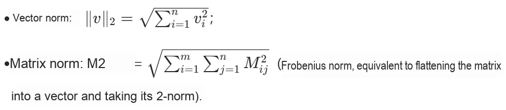
Example:
from ulab import numpy as np

vec = np.array([1,2,3])
mat = np.array([[1,2],[3,4]])
print("向量2-范数:", np.linalg.norm(vec))  # √(1+4+9)=√14≈3.7417
print("矩阵2-范数:", np.linalg.norm(mat))  # √(1+4+9+16)=√30≈5.4772
6.2.3 inv (matrix inversion)
- Core Restriction: The input must be a non-singular square matrix (determinant ≠ 0, no zero diagonal elements); otherwise, a
ValueErrorwill be raised. - Memory Optimization: Primarily based on in-place computation, the additional memory required is only float type equivalent to twice the number of elements in the original matrix, which adapts to the limited RAM of embedded systems;
- Time-consuming characteristics: It grows with the matrix dimension, but is not strictly linear due to the overhead of function calls (input checking, memory allocation)(only ~299 us for an 8x8 matrix).
6.3 Core Differences Between ulab and numpy
| Dimension | ulab | numpy |
|---|---|---|
| Matrix type support | eig supports only real symmetric matrices; only real matrices are supported overall | eig supports non-symmetric / complex matrices; all matrix types are supported |
| Norm functionality | Supports only the 2-norm, no parameters | Supports the ord parameter (1 / 2 / ∞ / Frobenius, etc. norms) |
| Exception handling | Raises ValueError if the input does not meet the conditions, with a concise message | More detailed error messages; in some cases returns a warning instead of an exception |
| Performance / memory | Optimized for embedded use (C implementation, low memory overhead) | Optimized for general-purpose platforms; strong performance on desktop but high overhead on embedded |
| Result consistency | Eigenvalue / eigenvector order / sign may differ (mathematically equivalent); results of other functions are identical | Stable results, fixed order / sign |
VII. Random Number Generation with ulab numpy.random
The numpy.random module of ulab only implements the Generator based on the PCG random algorithm (32/64-bit), which is lightweight-adapted focusing on three random number distributions frequently used in embedded scenarios, with the core features as follows.
7.1 Basics: Generator Object
Generator is the core carrier for generating random numbers, and all random number methods need to be called through instances. The core rules are as follows:
- Initialization: A single integer must be passed in as the seed (e. g.,
np.random.Generator (123456)). If the seed is fixed, the generated random number sequence will be completely fixed (reproducible, suitable for debugging/verification); - Underlying Algorithm: Based on the PCG random algorithm ( https://www.pcg-random.org/ ), it outperforms the traditional linear congruential algorithm;
- State properties: They are stateful Python objects that record the current state of the random number generator (consecutive calls to the method will generate different random numbers);
- Output type: All methods return by default an
float64-type ndarray (whensizeis specified) or a single floating-point number (whensize= None).
7.2 Three Major Random Number Methods: Comparison of Parameters and Functions
| Method | Distribution type | Core parameters | Key features (differences from numpy / other methods) |
|---|---|---|---|
| normal | Normal (Gaussian) distribution | loc=0.0 (mean), scale=1.0 (standard deviation), size=None (output shape) | ① Implemented internally with the Box-Muller transform; ② Supports calls with positional / keyword arguments; ③ No out parameter; ④ Core generation logic is identical to numpy.random.normal |
| random | [0, 1) uniform distribution | size=None (output shape), out=None (output array) | ① The only method that supports the out parameter (core embedded optimization); ② out must be a float ndarray; a conflict between size and the shape of out raises an exception; ③ The out array can be reused to avoid repeated memory allocation; ④ Compared with numpy's random, keeps only core functionality, with fewer extension parameters |
| uniform | [low, high) uniform distribution | low=0.0 (lower bound), high=1.0 (upper bound), size=None (output shape) | ① No out parameter; ② With low=0 and high=1, generates exactly the same sequence as random; ③ Supports custom intervals, making up for the fixed interval of random; ④ Supports calls with positional / keyword arguments |
7.3 Key Usage Examples and Notes
7.3.1 Fix the seed to ensure result reproducibility
During debugging in embedded scenarios, a fixed seed ensures that the random number sequence remains completely consistent, which facilitates problem localization:
from ulab import numpy as np

# Same seed → same random number sequence
rng1 = np.random.Generator(123456)
rng2 = np.random.Generator(123456)

print(rng1.normal())  # -6.285246229407202
print(rng2.normal())  # Exactly the same result
7.3.2 Reuse of out array by random
Embedded devices have limited RAM, so reusing the out array can reduce memory allocation and deallocation overhead:
from ulab import numpy as np

rng = np.random.Generator(123456)
# Preallocate a float64 array as a buffer
buf = np.zeros((3,3), dtype=np.float)

print("复用前的缓冲区:\n", buf)
# Write random numbers directly into the buffer, no new array created
rng.random(out=buf)
print("复用后的缓冲区:\n", buf)
7.3.3 Equivalence of uniform and random
uniform is random in its general form, and the two are completely equivalent under default parameters:
from ulab import numpy as np

rng = np.random.Generator(123456)
# When low=0 and high=1, uniform is equivalent to random
print(rng.random(size=(2,2)))        # [0,1) uniform distribution
print(rng.uniform(0, 1, size=(2,2))) # Generates exactly the same sequence
7.3.4 Core Differences Between ulab and Standard NumPy
| Dimension | ulab | numpy |
|---|---|---|
| Generator support | Supports only the PCG algorithm Generator | Supports multiple random number generators such as PCG, MT19937, Philox |
| Distribution type | Supports only normal distribution, [0,1] uniform distribution, and custom-interval uniform distribution | Supports dozens of distributions (Poisson, exponential, binomial, etc.) |
| Parameter richness | Minimal method parameters, keeping only core functionality: • random: only size / out • uniform: no out • normal: no out / dtype | Complete parameter system: • Supports dtype to specify the output type • All methods support the out parameter • Supports multithreading / vectorization optimization |
| Memory optimization | The out parameter of random is designed specifically for memory-constrained embedded scenarios | Supports more general memory optimizations, but has no embedded-specific adaptation |
| Compatibility | Core parameters (size / loc / scale / low / high) are the same as numpy | Fully compatible with the numpy API, supports extension parameters and advanced features |
VIII. Integration with ulab scipy.integrate
The scipy.integrate module of ulab is a lightweight subset of CPython's scipy.integrate. Its algorithms are not directly ported; instead, they are optimized and implemented based on embedded resources, retaining only 4 core numerical integration functions. The core features are as follows:
8.1 Basic Module Configuration (Prerequisite: Must Be Met First)
This module is not enabled by default and needs to be enabled by modifying the compilation macro in ulab.h, and its precision is strongly correlated with the floating-point configuration:
| Configuration item | Purpose | Recommended value (embedded) |
|---|---|---|
| ULAB_SCIPY_HAS_INTEGRATE_MODULE | Enable the entire integration module | 1 (enabled) |
| ULAB_INTEGRATE_HAS_QUAD / ROMBERG / SIMPSON / TANHSINH | Enable the corresponding integration function individually | Enable as needed (reduces firmware size) |
| MICROPY_OBJ_REPR_A + MICROPY_FLOAT_IMPL_DOUBLE | Enable float64 precision | 1 (preferred, higher precision) |
| Error tolerance (eps) | Default error threshold of each integration function | float64: 1e-14; float32: 1e-8 |
Key Limitations: All functions do not support complex integration, but can be extended based on existing functions (e. g., integrating the real part and imaginary part separately after splitting).
8.2 Four Major Integral Functions: Comparison of Core Parameters and Characteristics
| Function | Implemented algorithm | Core parameters (required + optional) | Return value | Applicable scenarios | Compared with CPython scipy Key differences |
|---|---|---|---|---|---|
| quad | Adaptive Gauss–Kronrod (G10, K21) integration | Required: f (callable function), a / b (lower / upper integration limits) Optional: order=5 (integration order), eps=default value (error tolerance) | (integration result, error estimate) (two floats) | General-purpose numerical integration (first choice in most scenarios) | CPython wraps QUADPACK (automatic switching among multiple algorithms); ulab implements only Gauss–Kronrod |
| romberg | Romberg integration (Newton–Cotes extrapolation) | Required: f, a / b Optional: steps=100 (number of sampling steps), eps=default value | A single float (integration result only) | Suited to integrands that are smooth, have continuous derivatives, and are sampled at equal spacing | Deprecated in CPython 1.12+; still kept in ulab; no error estimate returned |
| simpson | Adaptive Simpson integration | Required: f, a / b Optional: steps=100, eps=default value | A single float (integration result only) | Routine integration with moderate accuracy requirements | CPython requires passing an array of function values; ulab adapts the sampling interval automatically |
| tanhsinh | Optimized double-exponential (DE) integration (Tanh-Sinh / Sinh-Sinh / Exp-Sinh) | Required: f, a / b Optional: levels=6 (number of iteration levels), eps=default value | (integration result, error estimate) (two floats) | Endpoint singularities, infinite derivatives, or infinite integration intervals (such as Gaussian integrals) | CPython exposes the interface only from 1.15+; ulab is an optimized implementation; the only one that supports infinite integration limits |
8.3 In-depth Analysis of Key Functions
8.3.1 quad: General Preferred
- Algorithm advantages: It can adjust sampling points through Self-Adaptation, balancing accuracy and efficiency, making it a "universal" choice for embedded scenarios;
- Core parameters:
order— the higher its value, the higher the integration order, the better the accuracy but the slightly longer the processing time (the default value 5 is sufficient for most scenarios);
Example (fix UsageError in the document, correct MicroPython code):
from ulab import scipy

# Define the integrand: f(x) = x² + 2x + 1
def f(x):
    return x**2 + 2*x + 1

# Integration interval [0,5], order 5, error tolerance 1e-10
result, error = scipy.integrate.quad(f, 0, 5, order=5, eps=1e-10)
print(f"积分结果 = {result}, 误差估计 = {error}")
# Theoretical value: ∫(0→5) (x+1)² dx = ( (5+1)³ - (0+1)³ )/3 = (216-1)/3 ≈ 71.66666666666667
8.3.2 tanhsinh: Handling Special Integrals (Infinite Limits / Singular Points)
- It is the only one that supports infinite integration limits (
-np.inf/np.inf), making it the sole option for scenarios such as Gaussian integration; - Example (Gaussian integral, theoretical value √π ≈ 1.77245385091):
from ulab import scipy, numpy as np
from math import exp, sqrt, pi

# Gaussian integral function: f(x) = e^(-x²)
def f(x):
    return exp(-x**2)

# Integration interval (-∞, +∞)
result, error = scipy.integrate.tanhsinh(f, -np.inf, np.inf)
print(f"积分结果 = {result}, 误差估计 = {error}")
print(f"理论值 = {sqrt(pi)}")
8.3.3 Romberg/Simpson: Supplementary Scenarios
romberg: Equally-spaced sampling, suitable for scenarios requiring fixed sampling points (such as integration of hardware sampling data), but it has been deprecated in CPython and only retained in ulab;simpson: Self-Adaptation sampling, with accuracy slightly lower than that ofquad, yet taking slightly less time, which is suitable for fast integration with low accuracy requirements;
Example (simpson):
from ulab import scipy

def f(x):
    return x**2 + 2*x + 1

# Integration interval [0,5], default steps=100
result = scipy.integrate.simpson(f, 0, 5)
print(f"辛普森积分结果 = {result}")
8.3.4 Notes on Performance and Accuracy
- Floating-point precision selection: float64 (
MICROPY_FLOAT_IMPL_DOUBLE) is enabled by priority; float32 is available but will lead to a significant increase in error (the default eps drops from 1e-14 to 1e-8); - Parameter trade-off:
steps/levels/order— the higher their values, the better the accuracy, but the time consumption and memory usage will increase slightly (a balance is required for embedded scenarios); - Time consumption reference: On embedded devices (e. g. pyboard), the time consumption order of the 4 functions is:
romberg<simpson<quad<tanhsinh(tanhsinh takes the longest time due to the maximum number of iteration layers).
IX. Solving Linear Systems with ulab scipy.linalg
The scipy.linalg module of ulab only implements two linear system solving functions for "special matrices", serving as a supplement to numpy.linalg, and is designed for efficient computing in embedded scenarios (solving triangular matrices / Cholesky decomposed matrices is more efficient than general matrix inversion), with its core features as follows.
9.1 Core Comparison of Two Functions
| Function | Core function | Input parameters | Key rules | Core differences from CPython scipy |
|---|---|---|---|---|
| cho_solve | Given the Cholesky decomposition matrix L of a known matrix A (A = LLᵀ), solve the linear system Ax = b | Required: ① L: lower-triangular matrix from the Cholesky decomposition (ndarray) ② b: right-hand-side vector of the system (ndarray) | 1. L must be the correct lower triangular matrix from the Cholesky decomposition; otherwise the result is meaningless; 2. Returns the solution vector x directly (float64 ndarray); 3. No extra parameters; fixed computation path and minimal logic | CPython requires an (L, lower) tuple to specify upper/lower triangular explicitly; ulab takes the decomposed matrix directly and omits the redundant parameter, giving a simpler interface |
| solve_triangular | Assuming matrix A is triangular (upper / lower), solve the linear system Ax = b | Required: ① A: matrix (ndarray) ② b: right-hand side vector (ndarray) Optional: lower=False (default is upper triangular; True means lower triangular) | 1. A does not need to be explicitly triangular; the function automatically ignores elements outside the specified triangular region (treated as 0); 2. A·x = b holds only when A is actually triangular; 3. Returns the solution vector x (float64 ndarray) | 1. CPython supports more parameters (such as unit_diagonal, overwrite_b); ulab keeps only the core lower parameter; 2. ulab handles non-triangular matrices more leniently: it does not raise an error, but the result may deviate |
9.2 In-depth Analysis of Key Functions
9.2.1 cho_solve: Efficient Solution after Cholesky Decomposition
- Core prerequisite: You must first obtain the Cholesky decomposition matrix L of matrix A (A is required to be a positive definite symmetric square matrix) via
numpy.linalg.cholesky; otherwise, the result ofcho_solvecarries no mathematical significance.

Full Usage Example:
from ulab import numpy as np
from ulab import scipy as spy

# 1. Define a symmetric positive definite matrix A (prerequisite for Cholesky decomposition)
A = np.array([[25, 15, -5], [15, 18, 0], [-5, 0, 11]])
# 2. Cholesky decomposition gives the lower triangular matrix L
L = np.linalg.cholesky(A)
# 3. Define the right-hand side vector b of the system of equations
b = np.array([10, 20, 30])

# 4. Solve Ax = b
x = spy.linalg.cho_solve(L, b)
print("解向量x:", x)

# 5. Verify: LL^T x should equal b (A=LL^T)
LT = L.T  # Transpose to get the upper triangular matrix
verify = np.dot(np.dot(L, LT), x)
print("验证 LL^T x = b:", verify)  # Output is close to [10,20,30] (floating-point error)
9.2.2 solve_triangular: Dedicated Solver for Triangular Matrices
- Core Pitfall: The function does not verify whether the input matrix is a triangular matrix, and only extracts the corresponding triangular region (treating the remaining elements as 0) according to the
lowerparameter to compute the solution x. Only when the input is a genuine triangular matrix does the relation dot (A, x)= b hold; - lower parameter logic:
lower= False(default): only use the upper triangular region of the matrix (the diagonal and above), and the lower triangle is treated as 0;lower= True: only use the lower triangular region of the matrix (the diagonal and the part below it), and treat the upper triangular part as 0;
Example of pitfalls (verifying the issue of non-triangular matrices):
from ulab import numpy as np
from ulab import scipy as spy

# Non-lower-triangular matrix (upper triangular elements deliberately scrambled)
a = np.array([[3, 2, 1], [2, 1, 0], [1, 0, 1]])
b = np.array([4, 2, 4])

# Solve with lower=True (uses only the lower-left triangle, ignores upper triangular elements)
x = spy.linalg.solve_triangular(a, b, lower=True)
print("解向量x:", x)  # [1.333, -0.666, 2.666]

# Check 1: direct dot(a, x) ≠ b (because a is not a lower triangular matrix)
print("dot(a, x):", np.dot(a, x))  # [5.333, 1.916, 3.666]

# Check 2: take only the lower-left triangle of a (remove the part treated as 0), and the dot result equals b
a_lower = np.array([[3, 0, 0], [2, 1, 0], [1, 0, 1]])
print("dot(左下三角a, x):", np.dot(a_lower, x))  # [4.0, 2.0, 4.0]
9.2.3 Advantages of Application in Embedded Scenarios
- Better performance: Solving triangular matrices / Cholesky decomposition matrices does not require full matrix inversion, and the computational load is much smaller than that of
numpy.linalg.inv; on embedded devices (e. g. pyboard), the time consumption can be reduced by more than 50%; - Lower memory usage: There is no need to store the complete matrix after inversion, and only the elements in the triangular region need to be processed, which adapts to the limited RAM of embedded systems;
- Extremely streamlined logic: remove extended parameters of scipy (such as
overwrite_b/unit_diagonal), retain only core functions to reduce firmware size.
X. Root Finding for Univariate Functions with ulab scipy.optimize
The scipy.optimize module of ulab only implements three univariate optimization functions that are frequently used in embedded scenarios. Its core logic is "iterative loops implemented at the C layer + custom functions called at the Python layer", which delivers roughly 2x faster performance than pure Python (far lower than the performance improvement of ulab's vector operations). Its core features are as follows.
10.1 Core Comparison of the Three Major Functions
| Function | Core function | Required parameters | Optional control parameters | Return value | Underlying algorithm | Key features (advantages / limitations) | Performance (vs pure Python) |
|---|---|---|---|---|---|---|---|
| bisect | Root finding for a single-variable function (solve f(x)=0) | ① f (single-argument callable) ② a / b (interval endpoints, must satisfy f(a)·f(b) < 0) | xtol=2.4e-7 (root precision) maxiter=100 (maximum iterations) | Root location (float) | Bisection method | ✅ Very robust (low requirement on initial value) ❌ Slow convergence (linear convergence) | About 2× faster. Example: Python ~1270 μs → C ~642 μs |
| fmin | Minimization of a single-variable function (solve min f(x)) | ① f (single-argument callable) ② x0 (initial value) | xatol (x convergence precision) fatol (function value precision) maxiter (maximum iterations) | Minimum location (float) | Downhill simplex method (Nelder–Mead) | ✅ No derivatives needed, robust ❌ Single variable only (scipy supports multiple variables) | About 2× faster (core iteration implemented in C) |
| newton | Root finding for a single-variable function (solve f(x)=0) | ① f (single-argument callable) ② x0 (initial value) | tol (absolute tolerance) rtol (relative tolerance) maxiter (maximum iterations) | Root location (float) | Newton–Raphson method (derivative estimated numerically and automatically) | ✅ Fast convergence (quadratic convergence) ❌ Sensitive to initial value (must be close to the true root) | About 2× faster (iteration logic implemented in C) |
10.2 In-depth Analysis of Key Functions
10.2.1 bisect (bisection method for root finding) - robust and preferred
- Core Rule: The condition
f (a)⋅f (b)<0(i. e., the function values at the two endpoints have opposite signs) must be satisfied; otherwise, aValueErrorwill be raised directly. - Parameter Trade-off:
xtolis smaller, the higher the accuracy of the root will be, yet the more iterations are required and the longer the computation time will be;maxiterThe smaller its value, the earlier the iteration will terminate, the lower the accuracy will be, yet the shorter the time consumption will be;
Complete runnable example:
from ulab import scipy as spy

# Define the root-finding function: f(x) = x² - 1 (roots at x=1 and x=-1)
def f(x):
    return x**2 - 1

# Basic usage: find the root in the interval 0~4 (expected ≈1.0)
root_basic = spy.optimize.bisect(f, 0, 4)
print(f"基础用法根位置:{root_basic}")  # 0.99999976 (close to 1.0)

# Limit the number of iterations (8): precision decreases
root_iter = spy.optimize.bisect(f, 0, 4, maxiter=8)
print(f"8次迭代根位置:{root_iter}")  # 0.984375

# Relax the precision (0.1): faster but less precise
root_tol = spy.optimize.bisect(f, 0, 4, xtol=0.1)
print(f"0.1精度根位置:{root_tol}")  # 0.9375
10.2.2 fmin (Downhill Simplex Method for Minimum Finding) - Derivative-Free Minimum Finding
- Core Advantages: No need to compute function derivatives (manual derivative derivation is not required in embedded scenarios, reducing development costs);
- Parameter Logic: Stop iteration when either
|x_new - x_old| < xatolor|f (x_new) - f (x_old)| < fatolis satisfied;
Complete runnable example:
from ulab import scipy as spy

# Define the minimum-value function: f(x) = (x-1)² - 1 (minimum at x=1, function value=-1)
def f(x):
    return (x-1)**2 - 1

# Initial value 3.0, default precision
min_x = spy.optimize.fmin(f, 3.0)
print(f"默认精度最小值位置:{min_x}")  # 0.9996 (close to 1.0)

# Relax the x precision (0.1): result deviates slightly but is faster
min_x_tol = spy.optimize.fmin(f, 3.0, xatol=0.1)
print(f"0.1精度最小值位置:{min_x_tol}")  # 1.2 (acceptable within the precision range)
10.2.3 Newton (Newton-Raphson root-finding) — Fast Converging Root-Finding
- Core Features: Automatically estimates the derivative of a function (no need to manually derive the derivative function), with a convergence rate much faster than the bisection method, but it is sensitive to the initial value (it will not converge if the initial value is too far from the real root);
- Parameter Logic:
tol(absolute tolerance) andrtol(relative tolerance) jointly control convergence, and the iteration stops when|x_new - x_old| < tol + rtol*|x_new|is satisfied;
Complete runnable example:
from ulab import scipy as spy

# Define the root-finding function: f(x) = x³ - 2 (root at x=∛2 ≈1.2599)
def f(x):
    return x**3 - 2

# Initial value 3.0, absolute tolerance 0.001, relative tolerance 0.01
root = spy.optimize.newton(f, 3.0, tol=0.001, rtol=0.01)
print(f"牛顿法根位置:{root}")  # 1.2601 (close to the true value)
10.3 Core Differences from CPython scipy
| Dimension | ulab | CPython scipy |
|---|---|---|
| Variable support | Single-variable functions only | Supports single- and multi-variable functions |
| Parameter richness | Keeps only core control parameters (precision / iterations) | Supports extended parameters (such as full_output for detailed output, callback) |
| Algorithm extensions | newton supports only automatic numerical derivative estimation (cannot be passed manually) | newton supports passing a derivative function manually, and can select the secant method / Halley's method |
| Performance optimization | C optimization for embedded scenarios (small size, low memory usage) | General optimization for desktop (full-featured, but high overhead for embedded) |
11. ulab scipy.signal.sosfilt Second-order IIR Filter
11.1 Brief Introduction
The sosfilt in ulab is a lightweight subset of CPython's scipy.signal.sosfilt. It retains only the core logic of cascaded second-order sections (SOS) IIR filtering for 1D signals, which is frequently used in embedded scenarios, and is implemented using the direct-form II transposed structure (to avoid numerical precision loss in high-order filters), adapting to the requirements of low memory footprint and small size for embedded systems.
Brief Introduction to IIR Filtering
The core of IIR filtering lies in its recursion structure, which calculates the current output by leveraging past outputs and the input. This structure defines its core advantages and disadvantages, and also serves as the key to scenario selection:
- ✅ Advantages: With the same filtering effect, its order is much lower than that of FIR (e. g., a 10th-order IIR is roughly equivalent to a 100th-order FIR), featuring small computation load and extremely low memory usage; it can achieve "steep filtering characteristics"(high roll-off) with a low order.
- ❌ Disadvantages: phase nonlinearity (non-constant group delay); high-order IIR filters are prone to numerical instability (however, ulab's
sosfiltcan avoid this issue by splitting the filter into second-order sections (SOS)).
Applicable to:
- Embedded devices with low computing power / resource constraints (the core scenario): The core of IIR filtering lies in its recursion structure, which calculates the current output by combining the past outputs and the input — this defines its core advantages and disadvantages, and also serves as the key to scenario selection:
- ✅ Advantages: With the same filtering effect, its order is much lower than that of FIR (e. g., a 10th-order IIR is roughly equivalent to a 100th-order FIR), featuring small computation load and extremely low memory usage; it can achieve "steep filtering characteristics"(high roll-off) with a low order.
- ❌ Disadvantages: phase nonlinearity (non-constant group delay); high-order IIR filters are prone to numerical instability (however, this can be avoided by the
sosfiltfunction in ulab which implements second-order section (SOS) decomposition).
- Signal processing scenarios with extremely high real-time requirements: IIR filters do not require caching a large amount of historical input data (while FIR filters need to cache Nth-order inputs), and can complete calculations with only a small number of delay values, delivering extremely fast real-time response:
- Applicable Scenarios: For instance, when processing sensor signals with a 1kHz sampling rate, the per-frame computation time of an IIR filter is less than 100μs, enabling zero-latency "acquisition - filtering - output" operation; in contrast, if a 100th-order FIR filter is used, the total time for buffering plus computation will increase significantly.
- Practical Example:
- Real-time current/voltage filtering in industrial control (requiring immediate feedback control);
- Real-time smoothing of robot joint angles and drone attitudes (millisecond-level response required);
- Real-time triggering of smart home sensors (such as filtering and debouncing of human body infrared signals).
- Scenarios requiring "steep filtering characteristics"(narrowband / high roll-off): IIR filters can achieve "steep frequency roll-off" with an extremely low order (for example, to filter out 50Hz power-line noise, a 4th-order IIR alone can deliver a roll-off of 80dB per decade), while an FIR filter would require hundreds of orders to achieve the same effect, which is completely unaffordable for embedded systems:
- Applicable Reason: IIR filters are designed based on poles and zeros (including Butterworth, Chebyshev, and elliptic filters), which inherently fit the narrowband filtering requirement of "precisely filtering out a specific frequency band while retaining the target frequency band".
- Practical Example:
- 50/60Hz power frequency filtering for power signals (to filter out grid interference);
- Low-pass / high-pass filtering of audio signals (e. g., retaining the 200-3000Hz human voice frequency band while filtering out high-frequency noise);
- Resonance peak filtering for vibration sensors (precisely filtering out the single frequency of mechanical resonance).
- Scenarios insensitive to phase distortion: IIR features non-linear phase (i. e., different frequency components of a signal experience different delays), but in many scenarios, only the "amplitude" rather than the "phase" is a concern, making this characteristic fully acceptable:
- Applicable reason: Phase distortion does not affect the core information of the signal (such as amplitude and trend).
- Practical Example:
- Filtering of static/slowly varying signals (temperature, pressure, humidity): such signals change slowly, so the phase delay is negligible;
- Amplitude detection applications (e. g., signal strength, peak detection): only accurate amplitude is required, with no need to concern about the phase;
- Switching value trigger scenarios (e. g., judging whether the threshold is exceeded after filtering): The phase does not affect the threshold judgment.
Only with clear boundaries can you better select a model. In the following scenarios, FIR should be preferred over IIR:
- For scenarios with strict requirements for phase linearity (such as audio playback, communication signal demodulation, radar/ultrasonic ranging): FIR filters can be designed to have linear phase, while IIR filters cannot achieve this;
- High-order scenarios that require "absolute stability" and cannot split second-order sections: Although ulab's
sosfiltavoids instability with SOS, there is still numerical risk in very high-order IIR. - Multi-dimensional signal filtering (the
sosfiltin ulab only supports one dimension, and the multi-dimensional implementation of IIR is complex): FIR is easier to extend to multiple dimensions.
scipy.signal.sosfilt (sos, x, zi= None) applies a cascaded second-order IIR filter defined by sos to the uniformly sampled one-dimensional signal x, and returns the filtered data (along with optional final delay values).
| Parameter | Type requirements | Core rules |
|---|---|---|
| sos (required) | 2D float ndarray, shape (n_sections, 6) | ① Each row corresponds to one second-order section, in the format [b0, b1, b2, a0, a1, a2] (the first three are numerator coefficients, the last three are denominator coefficients); ② a0 is usually set to 1 (avoids denominator scaling and reduces numerical error); ③ The number of sections n_sections determines the filter order (total order = 2 × n_sections); ④ Must be float type (ulab implicitly converts integers to float, but explicit specification is recommended). |
| x (required) | 1D float ndarray | ① Supports 1D data only (core ulab constraint, no axis parameter); ② The input should be a uniformly sampled signal sequence (such as sensor voltage, acceleration, etc.). |
| zi (optional) | 2D float ndarray, shape (n_sections, 2) | ① Must strictly match the number of sections in sos (n_sections rows, 2 columns), otherwise a shape exception is raised; ② Represents the initial delay state of each second-order section (the filter's "initial state"); ③ When not passed, defaults to all 0 (initial rest state). |
| Return value | Trigger condition | Type / shape |
|---|---|---|
| y | All call scenarios | 1D float ndarray, same length as x (filtered output signal) |
| zf | When zi is passed | 2D float ndarray, same shape as zi (final delay state after filtering, usable as zi for the next signal segment) |
Complete runnable example:
from ulab import numpy as np
from ulab import scipy as spy

# ========== 1. Basic usage (no initial delay zi) ==========
# Define SOS coefficients for 2 second-order sections (example coefficients; in practice generate them from the filter design)
sos = np.array([[1, 2, 3, 1, 5, 6], [1, 2, 3, 1, 5, 6]], dtype=np.float)
# 1D input signal
x = np.array([0, 1, 2, 3, 4, 5, 6, 7, 8, 9], dtype=np.float)

# Basic filtering (initial delay all zeros)
y = spy.signal.sosfilt(sos, x)
print("基础滤波结果 y:", y)

# ========== 2. Usage with initial delay zi ==========
# Define the initial delay (2 second-order sections, corresponding to 2 rows and 2 columns)
zi = np.array([[1, 2], [3, 4]], dtype=np.float)
# Filtering with initial delay
y_with_zi, zf = spy.signal.sosfilt(sos, x, zi=zi)
print("\n带初始延迟的滤波结果 y:", y_with_zi)
print("滤波结束后的最终延迟 zf:\n", zf)

# ========== 3. Continuous filtering (reuse zf as zi for the next segment) ==========
# New input signal segment
x_new = np.array([10, 11, 12], dtype=np.float)
# Use zf from the previous segment as the initial delay to ensure filtering continuity
y_new, zf_new = spy.signal.sosfilt(sos, x_new, zi=zf)
print("\n连续滤波结果 y_new:", y_new)
11.2 Core Differences from CPython scipy.signal.sosfilt
| Dimension | ulab | CPython scipy |
|---|---|---|
| Input dimensions | Supports 1D x only, no axis parameter | Supports N-D x, filter axis can be specified via axis |
| zi flexibility | Supports only the fixed shape (n_sections, 2) | Supports flexible shapes adapted to N-D x (such as (n_sections, ..., 2, ...)) |
| Feature extensions | No Array API support, no multiple backends (such as CuPy / PyTorch) | Supports the Array API standard, multiple backends, detailed exception messages |
| Memory / size | C implementation, suited to embedded, small size, low memory usage | Full-featured, but high overhead for embedded (not suitable for microcontrollers) |
| Numerical optimization | Keeps only core filtering logic, no extra numerical optimization | Includes various numerical optimizations, boundary handling and precision control |
11.3 Application Example: Power Frequency Filtering
In the following case, we first configure the core parameters: a sampling rate of 200 Hz and a Q factor of 50.
- Generate an analog mixed signal containing a 10Hz useful signal and 50Hz power frequency noise;
- A second-order IIR notch filter with a high Q factor is adopted, and the initial transient noise is eliminated through preheating.
from ulab import numpy as np
from ulab import scipy as spy
from math import sin, pi

# ===================== 1. Configure core parameters =====================
FS = 200.0
F0 = 50.0
DURATION = 1.0
N = int(FS * DURATION)
Q = 50.0

print("=== 1. Filter Configuration Parameters ===")
print(f"Sampling Rate (FS): {FS} Hz")
print(f"Target Notch Frequency (F0): {F0} Hz")
print(f"Signal Duration: {DURATION} s (Total Samples: {N})")
print(f"Notch Filter Quality Factor (Q): {Q}\n")

# ===================== 2. Generate simulated signal =====================
t = np.linspace(0, DURATION, N, endpoint=False)
useful_signal = np.array([sin(2 * pi * 10 * ti) for ti in t], dtype=np.float)
noise_50hz = np.array([0.5 * sin(2 * pi * 50 * ti) for ti in t], dtype=np.float)
mixed_signal = useful_signal + noise_50hz

print("=== 2. Original Signal Segments (First 10 Samples) ===")
print(f"Useful 10Hz Signal: {useful_signal[:10]}")
print(f"50Hz Power Frequency Noise: {noise_50hz[:10]}")
print(f"Mixed Signal (Useful + Noise): {mixed_signal[:10]}\n")

# ===================== 3. High-Q notch filter coefficients =====================
sos_notch_50hz = np.array([
    [0.970588235, 0.0, 0.970588235, 1.0, 0.0, 0.94117647]
], dtype=np.float)

print("=== 3. 50Hz Notch Filter SOS Coefficients ===")
print(f"SOS Matrix (shape: {sos_notch_50hz.shape}): {sos_notch_50hz}\n")

# ===================== 4. Filter warm-up (key fix: ensure consistent length) =====================
# Number of warm-up samples: first 10 points
warmup_len = 10
warmup_samples = mixed_signal[:warmup_len]
zi_warm = np.array([[0.0, 0.0]], dtype=np.float)
# Warm-up filtering: only obtain the stable delay values, discard the filtered results of the warm-up segment
_, zf_warm = spy.signal.sosfilt(sos_notch_50hz, warmup_samples, zi=zi_warm)

print("=== 4. Filter Warmup (Eliminate Initial Transient) ===")
print(f"Warmup Samples Length: {len(warmup_samples)}")
print(f"Stable Filter Delay After Warmup (zf_warm): {zf_warm}\n")

# ===================== 5. Main signal filtering (fixed concatenation logic) =====================
# Main signal: all 200 points (not with the first 10 removed), filtered using the delay values after warm-up
# This way the filtered signal length = 200, exactly the same as useful_signal
filtered_signal, _ = spy.signal.sosfilt(sos_notch_50hz, mixed_signal, zi=zf_warm)

print("=== 5. Filtered Signal Segment (First 10 Samples) ===")
print(f"Filtered Signal Length: {len(filtered_signal)}")
print(f"Filtered Signal: {filtered_signal[:10]}\n")

# ===================== 6. Verify filtering effect (no errors) =====================
noise_before = mixed_signal - useful_signal
noise_after = filtered_signal - useful_signal

rms_noise_before = np.sqrt(np.mean(noise_before[warmup_len:] **2))
rms_noise_after = np.sqrt(np.mean(noise_after[warmup_len:]** 2))
attenuation_ratio = (rms_noise_before - rms_noise_after) / rms_noise_before * 100

print("=== 6. Noise Reduction Effect ===")
print(f"RMS Noise Before Filtering: {rms_noise_before:.6f}")
print(f"RMS Noise After Filtering: {rms_noise_after:.6f}")
print(f"50Hz Noise Attenuation Ratio: {attenuation_ratio:.2f}%")
print(f"Stable Noise Residual (Last 10 Samples): {noise_after[-10:]}")
The output is as follows:
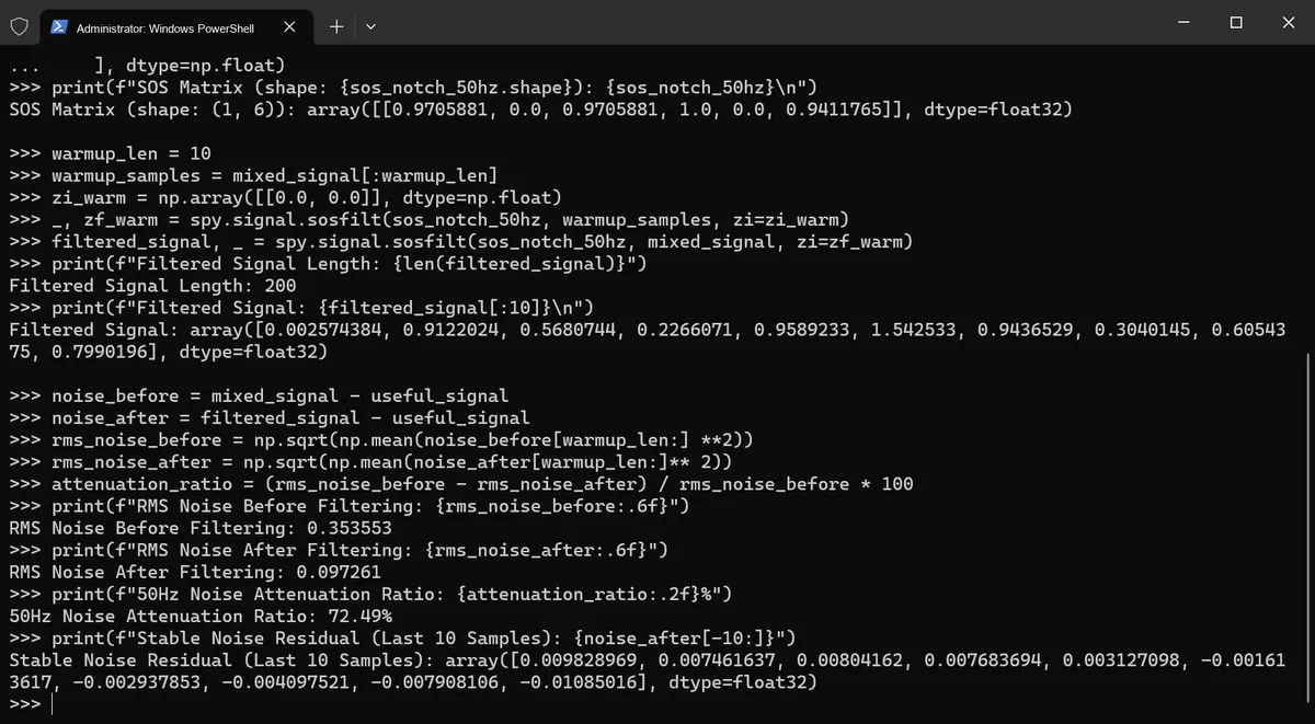
It can be seen that the RMS noise is 0.353553 before filtering and 0.097261 after filtering, with an attenuation rate of 72.49%, and the noise residue of the last 10 points in the stable section is less than 0.011.
12. ulab scipy.special Special Mathematical Functions
The scipy.special in ulab is a lightweight subset of the module with the same name in SciPy, which only implements 4 high-frequency special mathematical functions, with the core features:
- Input Compatibility: No modification to the call signature is required, and 3 types of inputs are supported:
- ✅ Scalars (e. g.,
5,3.2); - ✅ Scalar iterables (
range/list/tuple, e. g.range (9),[1,2,3]); - ✅ ulab
ndarray(one-dimensional / multi-dimensional; one-dimensional in the example).
- ✅ Scalars (e. g.,
- Output uniformity :
floattypendarrayregardless of input type (float64in the example, possiblyfloat32in embedded).
The four core functions of the module are as follows:
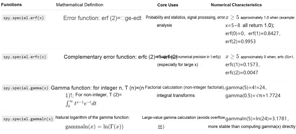
Complete runnable example:
from ulab import numpy as np
from ulab import scipy as spy

# Test gamma (gamma function)
x_scalar = 5  # Scalar input
x_list = [1,2,3,4,5]  # list input
x_ndarray = np.array([0.5, 1.5, 2.5])  # Non-integer ndarray input

print("=== gamma函数测试 ===")
print(f"gamma(5) (标量): {spy.special.gamma(x_scalar)}")  # 4!=24.0
print(f"gamma([1,2,3,4,5]) (list): {spy.special.gamma(x_list)}")  # [0!,1!,2!,3!,4!] = [1,1,2,6,24]
print(f"gamma([0.5,1.5,2.5]) (ndarray): {spy.special.gamma(x_ndarray)}")  # [√π≈1.772, √π/2≈0.886, 3√π/4≈1.329]

# Test gammaln (log gamma)
print("\n=== gammaln函数测试 ===")
print(f"gammaln(5): {spy.special.gammaln(5)}")  # ln(24)≈3.1781
print(f"gammaln([1,2,3]): {spy.special.gammaln([1,2,3])}")  # [ln(1),ln(1),ln(2)] = [0,0,0.6931]
13. ulab utils Module: Data Conversion and Spectrum Analysis
utils is a utility module designed by ulab specifically for embedded scenarios, which is not compatible with numpy, and it mainly addresses two pain points:
- ① Convert data in non-standard peripheral formats (e. g., 32-bit ADC signals) into ulab arrays;
- ② Memory fragmentation and high utilization issues during spectrum analysis.
13.1 Module Enable Method (compile macro must be configured)
utils module is not compiled into the firmware by default, you need to modify the macro in ulab.h:
// 1. Enable the entire utils module
#ifndef ULAB_HAS_UTILS_MODULE
#define ULAB_HAS_UTILS_MODULE               (1)
#endif

// 2. Enable specific functions (enable as needed to reduce firmware size)
#ifndef ULAB_UTILS_HAS_FROM_INT16_BUFFER   // 16-bit signed integer conversion
#define ULAB_UTILS_HAS_FROM_INT16_BUFFER    (1)
#endif
#ifndef ULAB_UTILS_HAS_FROM_UINT32_BUFFER  // 32-bit unsigned integer conversion
#define ULAB_UTILS_HAS_FROM_UINT32_BUFFER   (1)
#endif
// Other functions: from_int32_buffer/from_uint16_buffer/spectrogram work the same way
13.2 Core Functions
13.2.1 Buffer Conversion Function (from_(u) int16/32_buffer)
Directly convert the byte buffer of 16/32-bit integers output by peripherals (such as 32-bit sampling data from ADCs and microphones) into a ulab float -type ndarray, eliminating the need for manual byte parsing and integer concatenation, and adapting to embedded peripheral data formats.
| Parameter | Purpose | Embedded value |
|---|---|---|
| buffer (required) | Byte buffer (bytearray / bytes) | Connects directly to raw byte output of peripherals (such as the DMA buffer of an ADC) |
| count=-1 | Number of floats to convert (-1 means calculated automatically from buffer length) | Converts on demand, avoiding processing of redundant data |
| offset=0 | Skip the first N bytes of the buffer before converting | Ignore invalid data at the head of the buffer (such as peripheral frame header) |
| out=None | Writes the result into a predefined float array | Reuses memory, avoiding a new array on every conversion (solves insufficient embedded RAM) |
| byteswap=False | Whether to swap byte order | Adapts to endianness differences between peripheral and MCU (such as big-endian peripheral, little-endian MCU) |
13.2.1.1 Basic Conversion (No Parameters)
A 32-bit integer is formed by concatenating 4 bytes (in little-endian order: the lower byte comes first), and the difference between unsigned and signed conversions is reflected in the most significant bit (the sign bit).
from ulab import utils

# Byte buffer: 8 bytes = 2 32-bit integers (little-endian)
a = bytearray([1,1,0,0, 0,0,0,255])
# Unsigned conversion: 0x00000101=257, 0xFF000000=4278190080
print(utils.from_uint32_buffer(a))  # array([257.0, 4278190080.0])
# Signed conversion: 0xFF000000=-16777216 (two's complement)
print(utils.from_int32_buffer(a))   # array([257.0, -16777216.0])
13.2.1.2 Reusing the out Array (Memory Optimization)
On embedded devices, RAM is a scarce resource, so reusing arrays can prevent the fragmentation caused by frequent memory allocation and deallocation operations.
from ulab import numpy as np, utils

# Predefined float array (reuse memory, avoid creating a new one)
a = np.array([1,2], dtype=np.float)
b = bytearray([1,0,1,0, 0,1,0,1])
# Result is written directly into a, no new memory allocation needed
utils.from_uint32_buffer(b, out=a)
print(a)  # array([65537.0, 16777472.0])
13.2.1.3 Byte Order Swap (Peripheral Endianness Adaptation)
Solve the compatibility issue caused by the big-endian format of peripherals (such as some sensors) and the little-endian format of the MCU.
a = bytearray([1,0,0,0, 0,0,0,1])
# No swap: 0x00000001=1, 0x01000000=16777216
print(utils.from_uint32_buffer(a))          # array([1.0, 16777216.0])
# With swap: after byte reversal 0x00000001→1, 0x01000000→1 are exchanged
print(utils.from_uint32_buffer(a, byteswap=True))  # array([16777216.0, 1.0])
13.2.2 Spectrogram (High-efficiency Spectrum Analysis)
13.2.2.1 Function Orientation
Computing the power spectrum of a signal (the absolute value of the FFT) is equivalent to np.abs (np.fft.fft (signal)), but improves memory efficiency by more than 10 times — it eliminates multiple memory allocations during FFT, absolute value, and logarithmic operations.
13.2.2.2 FFT Compatibility Adaptation
ulab's FFT supports two modes, and spectrogram will automatically adapt to them:
| FFT mode | Input parameters | Equivalent logic |
|---|---|---|
| numpy compatible (recommended) | 1 argument (real or complex array) | np.abs(np.fft.fft(signal)) |
| Not numpy compatible | 2 arguments (real part + imaginary part) | np.sqrt(real**2 + imag**2) |
You can determine the FFT mode with the following code:
from ulab import numpy as np
if len(np.fft.fft(np.zeros(4))) == 2:
    print("FFT非numpy兼容(实虚部分开)")
else:
    print("FFT numpy兼容(复数输出)")
13.2.2.3 Core Parameters
| Parameter | Purpose | Embedded value |
|---|---|---|
| signal (required) | 1D real / complex array (signal to analyze) | Connects directly to sensor sampling data |
| scratchpad=None | Temporary buffer (length = 2 × signal length, float type) | Reuses temporary memory, avoiding a new allocation on every FFT |
| out=None | Writes the result into a predefined array | Reuses memory, reducing allocations |
| log=False | Whether to return the logarithmic power spectrum | Computed directly inside, avoiding a new array from np.log() |
13.2.2.4 Example Interpretation
Example 1: Basic Usage
from ulab import numpy as np, utils

x = np.linspace(0, 10, 1024)
y = np.sin(x)
a = utils.spectrogram(y)  # Equivalent to np.abs(np.fft.fft(y))
print(a)  # Power spectrum array (absolute values)
Example 2: Memory Reuse for High-Frequency Calls (Core Advantage of Embedded Systems)
from ulab import numpy as np, utils

n = 1024
t = np.linspace(0, 2*np.pi, n)
scratchpad = np.zeros(2*n)  # Temporary buffer allocated only once

# Method 1: memory-efficient (reuse scratchpad+out)
for _ in range(10):
    signal = np.sin(t)
    # Result is written into signal itself, scratchpad is reused, compute the logarithm directly
    utils.spectrogram(signal, out=signal, scratchpad=scratchpad, log=True)

# Method 2: memory-inefficient (new arrays created each time, prone to fragmentation)
for _ in range(10):
    signal = np.sin(t)
out = np.log(utils.spectrogram(signal)) # Creates 2 new arrays each time- Method 1: Allocate only once
scratchpad, reuse the resultingsignalarray, with no additional memory allocation; - Method 2: Create a new one in each loop
spectrogramresult array +np.logresult array. Frequent allocation/deallocation leads to memory fragmentation (a fatal issue for embedded systems).
13.2.3 Core Summary
| Core function | Core embedded value | Key advantages |
|---|---|---|
| Buffer conversion functions | Adapts to peripheral 32/16-bit integer data | Direct conversion, byte-order support, memory reuse |
| spectrogram | High-frequency spectrum analysis (e.g., audio / vibration detection) | Memory reuse, avoids fragmentation, built-in logarithm operations |
| Overall design | Suited to low-RAM / low-compute MCUs | No redundant memory allocation, implemented in C layer (fast) |
14. Core Optimization Techniques for ulab
All the following techniques are designed around the core pain points of "limited MCU computing power (no FPU / low main frequency), scarce RAM, and fatal memory fragmentation", with each technique accompanied by its principle, applicable scenarios, and practical implementation suggestions.
14.1 Prefer using ndarray over native iterable objects
ulab functions process ndarray by directly manipulating memory pointers at the C layer: given the C type of the array (e. g. uint8/float32), only a single round of loop traversal of the pointer for accumulation/computation is required, with no overhead from function calls or type conversion; whereas for native iterable objects such as lists and tuples, Python variables need to be extracted one by one → converted to numeric types → then computed, which is extremely inefficient.
Practical Comparison:
| Operation | Code example | Speed comparison |
|---|---|---|
| List sum | np.sum([1, 2, 3, 4, 5]) | Baseline (1×) |
| ndarray sum | a = np.array([1, 2, 3, 4, 5]); np.sum(a) | About 3× faster |
| Pure Python sum | sum([1, 2, 3, 4, 5]) | About 40× slower (no hardware / C-layer acceleration) |
- ✅ Data needs to be reused multiple times (e. g., multiple calculations of sum/mean/max): convert it to an ndarray first, as the one-time conversion cost can be offset by multiple subsequent calculations;
- ❌ Data only for single calculation: No need to convert to ndarray (the construction overhead of conversion outweighs the benefits of direct calculation).
14.2 Choose a reasonable dtype (core to memory saving)
The default dtype of ulab is float (float32/64, occupying 4/8 bytes), while data from embedded peripherals (such as ADCs/sensors) are mostly 8/16-bit integers. Using a smaller dtype can save 3 to 7 times RAM without sacrificing computational accuracy (e. g., for summation or finding maximum/minimum values).
| Data source | Recommended dtype | Memory savings | Notes |
|---|---|---|---|
| 8-bit ADC data | uint8 | 75% (8 → 1 byte) | Take care to avoid numeric overflow (uint8 maximum is 255) |
| 16-bit accelerometer | int16 | 50% (4 → 2 bytes) | Covers positive and negative range (-32768 ~ 32767) |
| Only min/max / sum needed | Match the bit width of the data source | 4 ~ 8 times | No float needed, integer computation is faster |
| Filtering / spectrum analysis | float32 | — | Floating-point precision needed, prefer float32 over float64 |
14.3 Optimize the Axis Order of Multidimensional Arrays (Place the Longest Axis at the End)
Rules for traversing multidimensional arrays in ulab: The outermost loop corresponds to the first axis, and the innermost loop corresponds to the last axis (the "fast axis"):
- Inner loop (last axis): The pointer only needs to perform "address + offset" with no additional computation;
- Outer loop (pre-order axis): Element addresses need to be recalculated, which incurs high overhead.
| Array shape | Code | Traversal efficiency | Reason |
|---|---|---|---|
| Efficient | a = np.array(range(2000)).reshape((2, 1000)) | Fast | Last axis length is 1000, inner loop is long, only 2 outer repositionings needed |
| Inefficient | b = np.array(range(2000)).reshape((1000, 2)) | Slow | Last axis length is 2, inner loop is extremely short, 1000 outer repositionings needed |
numpy automatically adjusts the axis order (placing the longest axis at the innermost position), whereas ulab uses a fixed axis order, so you need to manually place the longest dimension at the end.
14.4 Reduce Intermediate Products (Avoid Memory Fragmentation)
Compound expressions (e. g., b[1:: 2] = a[:-1] + a[1:]) generate temporary intermediate arrays, which consume RAM and cause fragmentation (in embedded systems without memory management, fragmentation will gradually deplete RAM); splitting such operations can avoid additional memory allocation.
| Style | Code | Memory overhead | Applicable scenarios |
|---|---|---|---|
| Inefficient (compound) | b[1::2] = a[:-1] + a[1:] | Creates a temporary array (a[:-1] + a[1:]) | Non-loop / one-time operation |
| Efficient (split) | b[1::2] = a[:-1]; b[1::2] += a[1:] | No temporary array (only reuses views) | Loop / high-frequency operation |
Additional Recommendations:
- Avoid frequent use of Boolean indexing (e. g.,
b = a[a<4]):a<4will generate a temporary Boolean array, so you need to callgc.collect ()regularly in loops to clean it up; - Reuse the
outparameter: for example,utils.spectrogram (signal, out= signal)directly overwrites the original array without allocating new memory.
14.5 Image/Array Scaling (Low-Resolution Sensor Adaptation)
For low-resolution data such as 8x8 thermal imaging, replace the interpolation function with slicing + element-wise operations (interp) to avoid intermediate products and adapt to embedded low-computing-power scenarios.
Practical Example:
from ulab import numpy as np

# 8x8 thermal imaging raw data
a = np.random.randint(0, 255, (8,8), dtype=np.uint8)
# Preallocate the scaled array (15x15, allocated only once)
b = np.zeros((15,15), dtype=np.uint8)

# Row interpolation: odd rows are filled with the mean of adjacent rows
b[1::2,::2] = a[:-1,:]    # First assign the previous row
b[1::2,::2] += a[1:,:]    # Accumulate the next row
b[1::2,::2] //= 2         # Compute the mean (no floating point)

# Column interpolation: odd columns are filled with the mean of adjacent columns
b[:,1::2] = a[:,:-1]
b[:,1::2] += a[:,1:]
b[:,1::2] //= 2
No temporary arrays are used throughout the process, only slice views are reused, resulting in the lowest RAM usage.
15. A Brief Analysis of the Underlying Implementation and Extension of ulab
The underlying core of ulab is the ndarray data structure, which adopts a right-aligned shape/strides design (the longest axis serves as the fast axis for the highest traversal efficiency). Data is stored in contiguous memory, and sparse arrays (such as slices) return views instead of copies by adjusting strides and offsets, which greatly saves embedded RAM.Its core operations are all adapted to low-computing-power scenarios: iteration supports two modes: unrolled loop (high-speed) and rewinding function (dimension-independent); broadcasting achieves compatibility for arrays of different shapes through dimension padding + zero-step size; type promotion prioritizes overflow prevention (e. g., small types are promoted to larger types in integer operations, uint16 + int16 is converted to float), balancing compatibility and embedded-specific features.
Extending ulab can be achieved through three steps: enabling user modules, writing C-layer functions (including input validation, array creation, data traversal and calculation, and result return), and binding the Python namespace; after compile, the custom functions can be invoked. For embedded optimization, the following core principles shall be followed: prioritize dense arrays and fixed dtypes to reduce overhead, reuse arrays to avoid memory allocation, split composite expressions to circumvent fragmentation, and maximize adaptation to the constraints of low computing power and limited RAM of MCUs.
| Key concept / operation | Core characteristics |
|---|---|
| ndarray structure | Right-aligned shape / strides, data pointer points to contiguous memory; includes metadata such as dtype / itemsize, supports multidimensional arrays |
| Memory layout | Dense arrays have no skipped elements; "sparse" arrays such as slices produce views via strides / offset without copying data |
| Iteration mechanism | Provides unrolled loops (high speed, fixed dimensions) and rewind functions (dimension-independent, saves Flash); both use the fast axis as the inner loop |
| Broadcasting mechanism | Lower dimensions are padded with 1; lengths in the same dimension must be equal or 1; elements are reused via zero strides, enabling computation between arrays of different shapes |
| Type promotion | If any operand is float, the result is float; integer operations promote from smaller type to larger type; uint16 + int16 automatically converts to float to prevent overflow |
| Extension procedure | Enable ULAB_USER_MODULE → write C function (validate input → create array → compute → return) → bind to namespace → compile firmware |
For this section, you can visit the following link:
https://micropython-ulab.readthedocs.io/en/latest/ulab-programming.html
Summary of links to relevant firmware, source code and documents
Source Code
https://github.com/v923z/micropython-ulab
ulab Firmware Download
https://github.com/v923z/micropython-builder/releases/tag/latest
Document
https://micropython-ulab.readthedocs.io/en/latest
https://micropython-ulab.readthedocs.io/en/latest/scipy-signal.html
https://docs.scipy.org/doc/scipy/reference/signal.html#module-scipy.signal
Version Record
Version Number | Revision Date | Modifier | Modify Content |
v1.0 | 2026-01-19 | Lee Eryong | Initial version, based on the release date 2026-01-19 (MicroPython v1.24.0). |