
A light sensor changes its numbers when you cover it. A pressure sensor reacts when you press it. That is a satisfying first step for a prototype, but it leaves a practical question: can the rest of the product rely on those numbers?
The next step is to connect three things: what happened at the sensor, what voltage reached the converter, and what the software displayed. We ran three bench experiments on a GraftPort-RP2040 controller with GraftSense ADS1015, ADS1219 and ADS1115 converter boards: a real light sensor first, then a controlled signal that is easier to explain, then a look at what averaging does to a changing input.
Start with a change you can explain
An analog sensor represents something in the world as a voltage. An analog-to-digital converter (ADC) turns that voltage into a number. It does not know whether the number means brightness, force or temperature.
That gap trips up real projects: a builder reads changing values from an ADC and cannot tell whether they are normal. Define the expected response before you interpret an unfamiliar number as success or failure.
Our first setup fed a GL5516 light-sensing module into AIN0 of the ADS1015 board. The RP2040 read the converter over I2C, GPIO 4 for data and GPIO 5 for clock. Start with the module's specified power connection and a shared ground, then make one deliberate change to the light reaching the sensor.
The program read channel 0 at address 0x48 every half second and printed raw counts and a calculated voltage. On the ±4.096 V scale, a 12-bit signed result converts as raw * 4.096 / 2048. Choosing that scale does not let a 3.3 V-powered input tolerate 4.096 V; the input must still stay within the ADC's supply range. (Our first program divided by 2047, so its displayed values were very slightly off.)
The terminal moved from near zero to about 1.37 V. That is evidence of a changing electrical reading. It is not a lux calibration, and it does not tell you how the sensor will behave behind a tinted window in an enclosure.
For your own prototype, write the physical action beside each reading: uncovered, covered, moved closer, or placed behind the intended window. If a result surprises you, measure the voltage at the ADC input before changing software. That separates "the sensor output did not change" from "the converter or code did not report the change."
Replace the unknown input with a controlled one
A sensor is affected by lighting, placement and the object being measured. A signal generator removes those unknowns for a bench check: you choose the electrical input and watch how the acquisition path responds.
For the ADS1219 board, which has two SMA input connectors, we drove AIN1 from a handheld signal generator. The program used gain 1, the internal 2.048 V reference and single-shot conversion at a configured 20 samples per second. The host waited between reads, so that setting is not a claim of 20 logged readings per second.
The terminal found the converter at 0x40, and the positive readings rose from about 886 mV to 1788 mV and fell again. That makes the data path visible: input connector, selected channel, raw result, voltage calculation. A moving curve alone cannot tell you the error, though. For a slow measurement, apply several known DC levels and compare against a reference instrument.
A plot can mislead even when the numbers are fine. Our first plot put raw counts and millivolts on the same vertical axis. Counts were in the millions and millivolts around a thousand, so the voltage trace hugged the bottom and looked stuck. Plot them separately before deciding a value is frozen.
A 24-bit output gives more possible codes than a 12-bit one. It does not by itself give 24 useful bits of accuracy in an assembly. The ADS1219 driver we used also needs signed-result handling before it can be trusted for negative differential values; our run only produced positive readings. Describe the measurement before choosing the converter.
Make sure the scale matches the signal
The ADS1115 shows the next piece: input selection and conversion range. Its four input pins share one converter, and the input multiplexer chooses which voltage, or which difference between two voltages, is measured.
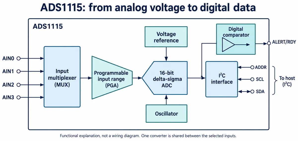
Single-ended measurement compares one input with ground. Differential measurement compares two inputs with each other. Neither removes the need to keep every pin inside its allowed operating range.
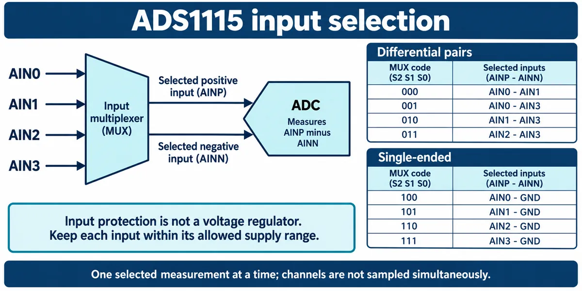
The configured range sets how much voltage one count represents. That helps turn a small sensor output into readable numbers, but it is separate from the supply limit. TI's ADS1115 datasheet describes both. The ±6.144 V range option is not permission to put 6 V on an input of a part powered from 3.3 V.
A Reddit r/AskElectronics thread shows the confusion: the author saw an almost fixed reading despite changing optical conditions and questioned the input voltage relative to the ADC supply. The cause was not settled in what we could read. Check the actual input voltage and range arithmetic before accepting any diagnosis.
A useful bench record keeps the ADC supply voltage, input channel, selected range, raw code and calculated volts together. A screenshot of a smooth line loses information you will need when the sensor moves into its final housing.
Keep the raw curve when you add averaging
For the ADS1115 averaging experiment we streamed two values side by side to SerialPlot: the raw sample and a moving average. This matters for interactive products, where a steady display is nice but a delayed response can feel wrong.
The program read I2C on GPIO 4 and 5 and sent binary frames on UART0 (GPIO 0 and 1) at 256000 baud, 8N1. Each frame starts with AA BB, followed by two little-endian 16-bit values: raw first, average second. The receiver must interpret them as signed values.
The average keeps the latest 20 readings and divides their sum by how many it holds:
window = []

def moving_average(sample, length=20):
    window.append(sample)
    if len(window) > length:
        window.pop(0)
    return sum(window) // len(window)
Apply it after acquiring a fresh sample, outside any timer callback, and log both values. Our acquisition helper read the previous conversion before starting the next, so the first value can be stale. A timer setting also does not prove the logging interval; record timestamps if response time matters.
The generator traces made the tradeoff plain. With a 5 Hz square wave, filtering softened the edges and delayed the response. With a 5 Hz pulse at 10% duty cycle, the moving average shrank the short pulse, which could hide the very event you wanted to detect. A triangle wave came out rounded and delayed. With a constant 3.0 V DC input, both traces settled together, which shows steady-state behavior but still not absolute accuracy without an independent comparison.
As a calculation only: a 20-sample average at an even 100 samples per second spans about 0.2 s and delays the signal by about 95 ms, and would strongly suppress a 5 Hz periodic component. These are properties of an ideal window, not timing we measured; our code requested a 10 ms timer period, while some captures showed different SerialPlot rate figures.
A slowly updated light-level display and a controller reacting to a quick hand movement should not share a filter just because it looks tidy.
Decide what the reading must let the product do
Before ordering a custom board, choose one behavior to verify: detecting a hand movement without noticeable delay, say, or distinguishing two conditions after the sensor is installed in its enclosure.
Then repeat the sequence with that behavior in mind: a known electrical input, then the actual sensor, then raw versus processed readings. Keep the intended cable, power source and housing in the later tests. Record what changed and how long the system took to respond, not just the cleanest graph.
A useful handoff includes the sensor model, board revision, a wiring photo, supply and range settings, the exact driver version, the raw log, and the physical condition behind each test. With those, you can tell whether the next fix belongs in sensor placement, the analog circuit, conversion code or filtering.